|
Paper: Fault Localization via Risk Modeling |
Background: Know:Failure analysis Recognize: Fault localization, risk modeling, MPLS, OSPF, backbone networks
Introduction[]
Path Fault:
Considering the MPLS network, MPLS labels are established between two edge routers along the shortest path identified by the underlying interior gateway protocol (IGP) such as OSPF or IS-IS. This architecture is currently used by many tier-1 ISP networks.
Failure scenario 1: When OSPF reroutes due to a change in IGP link weight, but MPLS does not update its label-switched paths accordingly. Therefore, all the packets belonging to that particular MPLS tunnel attempt to traverse the old path only to be dropped within the network.
Failure scenario 2: Configuration or operator error. For example, stuff may forget to enable MPLS on a newly added interface causing MPLS switched packets to be dropped at that interface.
Link Fault:
In the first scenario, the IP network has a construction of different routers on a basic point-to-point link between the optical topology (optical path). Monitoring alarm light circuit failure is usually in a separate basis, for example, a router failure appears to terminate in the router. Current best practice, you need to manually use a personal link failure notification to determine whether they have common network elements, such as routers. However, in the more complex scenario of failure, it is substantially more challenging to form a common group of individual alert, and it is often difficult to detect which layer a fault occurs in, such as a router in the transmission network of interconnected, or in the router itself.
[]
Path Fault:
In this problem, MPLS tunnels share individual IP links form the shared risks. Each individual link failure or degradation can affect all the MPLS tunnels simultaneously that ride through any particular link.
In practical, if there are multiple VPNs that ride through a given MPLS tunnel that rides through a failed link, all these VPNs are affected by a failure on that link. However, researchers mainly focus on the failure of MPLS tunnels, while noting that it can be extend arbitrarily into higher layers if need be.

b
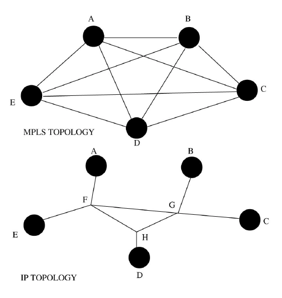
For example, in the figure below, edge nodes A-E are connected via intermediate nodes F-H. It is clearly that the set of paths A-F-G-B, A-F-G-C, E-F-G-C, and E-F-G-B (and the corresponding reverse paths) share a common link—the link from F to G. Hence, this link F-G forms a shared risk for this group of paths. But it should not include all the optical components and other SRLGs modelling for LINK FAULT in this context as MPLS failures do not involve optical components.
Path Fault:
A risk model can be setted up to indicated the set of the IP links that can be affected by the any component failure in the network. Multiple nodes can consist of the IP network topology by interconnecting links. The IP links that cover on top of an optical network can share share components in the network. Hence, it can share the risk in the network.
Normally, in tier-1 backbone networks, IP links are carried on opitical circuit, particularly use SONET. The network elements of opitical circuit system can provide the O-E-O conversion, protection/restoration to recover from opitical layer failures. In addition, a fiber span is that multiple opitical opitical fibers are carried in a single conduit.


Because every opitical component can carry multipe IP links, the physical elements such as fibers, fiber spans, and optical components can share risks. In addition to the optical compinents, our SRLG model also includes routers, modules, and ports. Moreover, physical components and logical software can be extended beyond.
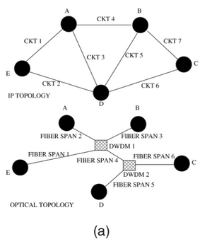
According to the figure (a), a network consists of 5 nodes which connected via 7 logical IP links that are routed over shared opitical layer components shown in the bottom of the figure (a).
Fault Localization Via Risk Modeling[]
Risk models are used to develop a fault localization methodology that can aid network operators in troubleshooting failures in an automated fashion.
The approach has three main components: Failure detection, risk modeling, the core localization algorithm and a set of refinements to handle domain-specific imperfections.
Failures detected at a higher layer (such as failed IP links or MPLS tunnels) are fed into a localization engine that spatially correlates these failures according to the risk model (based on the underlying topology) to identify a small set of likely locations of the failure. This localization step is the primary reconnaissance to a final—and often (necessarily) manual—step of actually diagnosing the root cause of the failure and fixing the problem.
Failure Detection and Risk Modeling
One of the two main inputs to a localization engine is the failure signature. The failure signature consists of a set of symptoms observed due to a given failure. The symptoms themselves are typically detected through explicit monitoring (either through probes or lower layer alarms).
For example, in order to check IP link integrity, each router in the network injects periodic “HELLO” messages to the router at the other end, which then acknowledges the receipt of the message. Considering the set of IP link failures that are temporally correlated (occur almost simultaneously) to constitute the failure signature in this scenario. Similarly, in monitoring MPLS tunnels for black holes, a monitoring server typically establishes connections (using, say, GRE tunnels) with each edge router and injects periodic probes to every other edge router in the network and reports if any of the probes are lost. Therefore, the set of origin/destination pairs (OD-pairs) that have lost connectivity (based on dropped probes) constitutes the failure signature in this scenario.
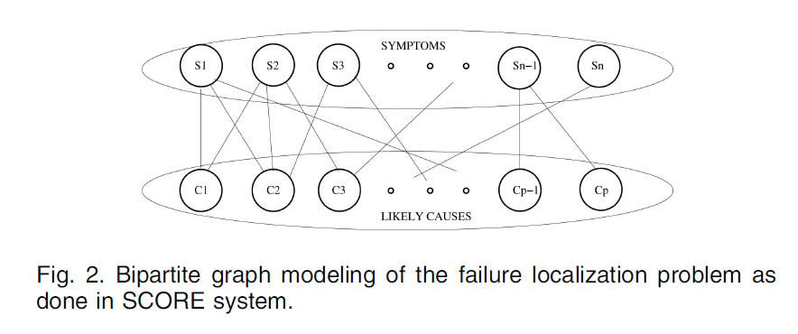
The other input required for fault localization is the risk model. Using a bipartite graph to represent the dependency between possible observable symptoms and correspondinglikely causes, as shown in Fig. 2. An edge exists between a symptom and a likely cause if that symptom can be observed given a failure in that root cause. As shown in Fig. 2, the top partition consists of the universal set of symptoms in the failure signature, and the bottom partition consists of the likely causes. Refering to the symptoms that have been reported by the failure detection system as observations.
In LINK FAULT, the symptoms are IP link failures and the likely root causes are the SRLGs such as fiber spans, optical amplifiers, etc.
In PATH FAULT, observations are failed MPLS tunnels, while the underlying IP links make up the potential root causes.
Fault Localization
Path Fault: The PATH FAULT example shows in figure below, if the set of paths A-F-G-B, A-F-G-C, E-F-G-C, and E-F-G-B all fail in a given time interval (temporally correlated failures), spatial correlation leads to the only link that is common to all these paths—the link from F to G. The localization engine would, therefore, return the singleton set {F-G} as the hypothesis in this failure scenario.
Link Fault:
Spatial correlation can be used for fault localization. The failure signature consists of a set of symptoms observed due to a given failure. The symptoms themselves are typically detected through explicit monitor- ing (either through probes or lower layer alarms). For an instance, according to Fig a, if CKT1 and CKT4 both fail at the same time, it is possible that the failure will be in the optical component DWDM1 because it is the only shared risk among these circuits (or IP links).
Using the core algorithm GREEDY to interatively pick SRLGs that are the best according to a metric.
updateSrlgStats(): computes this metric for all SRLGs
identifyCandidates(): picks the best SRLGs in the current iteration.
Algorithm 1. GREEDY(FailureSignatureF)
1: E={};
2: U=FailureSignatureF;
3: H={}; // Hypothesis set;
4: while (U={}) do
5: for (observationo = U) do
6: //ALL SRLGs for this obersavation o
7: srlgVector = getALLSRLGs(o);
8: //Update stats of SRLGs in srlgStatVector
9: updateSrlgStats(srlgVector);
10: end for
11: srlgSet = identifyCandidates();
12: //Move observations covered by SRLGs in srlgSet
13: //fromU to E
14: moveEvents (srlgSet,E,U);
15: addToHypothesis(H,srlgset);
16: end while
17:return H;
Managing Imperfections
1.Imperfections in Failure Signature and Risk Model
LINK FAULT suffers from relatively fewer imperfections, while PATH FAULT has many more sources of noise.
Path Fault:
The detection mechanism employed in PATH FAULT, on the other hand, consists primarily of endto-end probes that operate at a much lower frequency. So, for many reasonable failures, the failure signature is not complete. Of course, if the failure persists, eventually, all low-frequency probes that go through the failure are bound to detect the failure. But this means that we need to wait for a long time until the failure signature is complete.
Furthermore, because the topology is large (on the order of a million paths), any failure can affect a significant number of paths leading to an overwhelming number of observations and a large failure signature set. In order to operate in real time, the failure signature must occasionally be down sampled. Therefore, in this domain, the failure signature is expected to be largely incomplete. In addition to the incomplete failure signature, noise can cause some probes to be dropped in the network thus adding spurious observations to the failure signature.
The risk model in PATH FAULT for MPLS paths is primarily derived from the underlying IP topology. IP topology is inherently subject to churn due to various routing changes caused during failures, congestion, and maintenance activities. Therefore, the risk model needs to be computed on-the-fly for this scenario from the topology snapshots during the failure interval. Because the topology is extremely large, it is often impractical to construct the entire risk model; the fault localization algorithm needs to be designed to operate with a partial risk model.
Link Fault:
In link fault, lower layer alarms and high-frequency, touter-to-router probes can be used as the detection mechanism to detect losses in connectivity. Hence, detection of IP link layer faults is typically complete, in the sense that all IP links that fail due to a problem in the underlying optical network are detected with extremely high probability. Some fault messages are dropped during transmission, however, leading to a slightly incomplete failure signature.
The risk models for the large majority of optical networks are maintained through human-entered databases that may drift away from reality over time leading to occasional errors in the database. These errors can affect the localization results and must therefore be factored into the localization algorithm.
2.Handling Imperfections through Relaxed Metrics
In order to handle these imperfections using two different metrics to identify the candidate SRLGs in each iteration of the basic GREEDY algorithm.
Let Gi correspond to the ith shared risk in the network and jGij be the total number of observations that belong to the SRLG Gi. jGi \ Fj is the number of elements of Gi that also belong to F, the failure signature. We define hit ratio of the group Gi as jGi \ Fj=jGij. In other words, the hit ratio of a group is the fraction of elements in the group that are part of the failure signature. The coverage ratio of a group Gi is defined as jGi \ Fj=jFj, i.e., the fraction of the observation explained by a given risk group. If we have access to the complete failure signature and an accurate risk model, we can exploit the fact that every failed shared risk would have all associated observations in the failure signature. In other words, the hit ratio for the failed shared risks should be 1, so an optimal algorithm would select SRLGs with the highest coverage among those with a hit ratio of 1.
In the LINK FAULT, however, while we potentially have access to the entire failure signature and risk model, they are likely to contain a relatively small number of errors. In order to account for these errors,defining the SCORE algorithm that considers SRLGs with a hit ratio greater than a particular error threshold, which is generally slightly less than 1. I
n SCORE, the updateSrlgStatsðÞ routine computes the hit and coverage ratios, while identifyCandidatesðÞ routine picks the SRLG with the highest coverage ratio among those with hit ratio greater than the threshold.
On the other hand, if do not have access to the entire failure signature or associated risk model, then cannot compute a meaningful hit ratio for each and every SRLG in the first place. Therefore, in such situations, the greedy heuristic picks those SRLGs that have the highest coverage ratio in every iteration to output the hypothesis.
In the resulting algorithm MAX-COVERAGE, the identifyCandidatesðÞ routine is similar to that of SCORE algorithm, except the condition on the hit ratio is eliminated. Since the hit ratio is not required, the updateSrlgStatsðÞ routine does not need to compute it as well.
This algorithm, therefore, is applicable to PATH FAULT, where we can compute the coverage ratios of all the SRLGs but not the hit ratios.
In order to control the imperfections, two different metrics can be used to identify teh candidate SRLGs for teh GREEDY algorithm.
In link fault, when accessing to the failure signature and risk model, which may have few errors. We can define the SCORE algorithm to account for the number of errors.
If cannot access the to the failure signature or associated risk model, then can't compute a meaningful hit ratio for every SRLG in the first place.
3.Additional Refinements
While the relaxed selection metrics allow the localization algorithm to adapt to various operational realities, the localization architecture can supports further domain-specific refinements.
In particular, the input and the output from the localization algorithms can be postprocessed in order to better accommodate the needs of the particular domain. For instance, the error threshold is introduced to deal with the slight possibility of errors in the risk model for LINK FAULT; the choice of error threshold, however, is not immediately clear. Another problem is that the output may still contain several root causes, some of which exist because the algorithm is trying to explain each and every symptom that is input to the system.
This situation arises frequently in the PATH FAULT scenario and the output only the most significant root causes by effectively denoising the hypothesis. Another problem specific to the PATH FAULT domain is the need to consider multiple risk models as the fault can be result of either the old or new topologies.
System Architecture[]
3 required ingredients for fault localization can be listed below:
1). A failure detection system.
2). A risk model.
3). Localization algorithm.
Failure detection
Assumptions:
(a).A monitoring system produces a raw event steam continuously
(b).Path failure notifications are generated in response to the loss of end-to-end probes that constantly poll connectivity between various origin-destination paris.
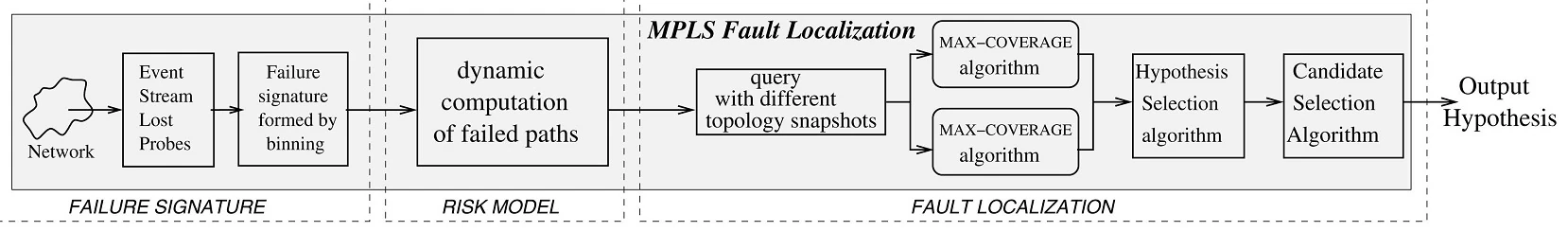

Fig1,System flow diagram for MPLS fault localization problems
Link Fault:
The failure signature upon which spatial correlation is applied is obtained from multiple kinds of network monitoring data sources relying on the particular failure scenario. In link fault, router syslogs can be used when it detects a link down.
A failure signature can be identified by clustering data source besed on discrete asynchronous. There are many different ways to cluster events. For link fault, we can use a clustering algorithm based on gaps between failure events. We consider the largest chain of events that are spaced apart by a set of threshold as potentially correlated events. Two events occur in a time period less than a given threshold, which can lead the same failure.
Path Fault:
Due to the presence of an excessive number of events attributable to noise in the network, a clustering scheme such as above results in clustering all events together into one cluster. Instead, we divide time into 15-minute bins.
The particular choice of the bin size is somewhat arbitrary and can be tuned in accordance with the typical duration of a failure event, required timeliness of diagnosis, and amount of evidence that needs to be collected.
Risk model[]
There are two key inputs to localization engine:
(1) Failure signature :consists of a set of symptoms observed due to a given failure
(2) Risk model:a bipartite graph to represent the dependency between possible observable symptoms and corresponding likely issues.
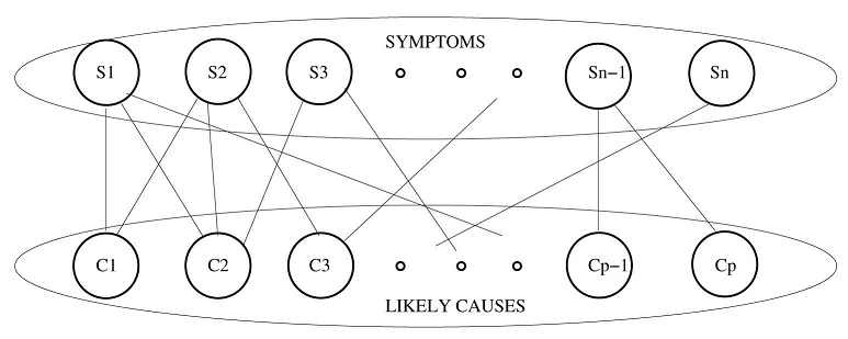
Fig.2.Bipartite graph modeling of the failure localization problem as done 'in SCORE system.
Observations are failed MPLS tunnels,while the underlying IP links make up the potential root causes.Only the paths for the OD-pairs are obtained instead of the entire topology for every snapshot.
Link fault:
In link fault, the risk model is consisted of disparate databases that can maintain for different types of shared risks. For example, optical layer shared risks that particular IP links traverse are extracted from databases populated from operational optical element management systems. Other risk groups are populated by periodically polling configurations from the various network elements. The underlying databases track the network and exhibit churn.Database churn can be coped with by regeneration risk groups multiple times.
Localization Algorithm[]
Path Fault:
Using the MAX-COVERAGE algorithm that iteratively selects the links covering the most observations in the failure signatures.
Two problems:
First, there can be potentially many different topology snapshots within a given failure interval and the question is which topology to use. To address this, first generating multiple hypotheses for a given failure signature using all the available topology snapshots in the failure interval, and use a hypothesis selection algorithm, called UNION, that outputs the union of hypotheses generated with each of the available topology snapshots.
By considering all possibilities, there is no loss in accuracy compared to an oracle that knows the ground truth (and hence, knows the right topology to pick), but precision is slightly lower.
Second, recall that the localization algorithm adds suspect links to the hypothesis until the hypothesis completely explains all the failed probes, including those observations that arise from inherent noise in the network. To address this, using a candidate selection algorithm (called ABSOLUTE) that removes candidate links from the hypothesis that explain fewer than a threshold number of observations, and thus, focuses only on the main links in the hypothesis.
Link Fault:
For the link fault, the Score algorithm can be queried with multiple error thresholds to get hypotheses that are different with each other. According to the figure 1, the hypothesis can be evaluated based on a cost function that relies on error threshold and the size of the hypothesis. Ratio between the size of the hypothesis and the threshold can be used as the cost, and the number of the hypothesis can be decreased by identifying cases where a small relaxation in the threshold.
Evaluation[]
Path Fault:
Metrics for Comparison:Define two primary metrics accuracy and precision for comparing our hypothesis with the ground truth.
(1) Accuracy:the fraction of the elements in the ground truth G also contained in the hypothesis H or |G∩H|=|G|. If G is a proper subset of H, then the accuracy is 1.
(2) Precision:quantity the size of the hypothesis in relation to the ground truth.It is defined as the fraction of elements in the hypothesis that are also present in the ground truth or |G ∩ H|=|H|. In effect, precision captures the amount of truth in the hypothesis.
Localization efficiency:the ratio of the number of suspect root-cause after localization to the numer before.
Building a simulator:
(1) Inject artificial failures that mimic real-life failure scenarios and obtain failures
(2) Apply localization algorithm to evaluate the accuracy
(3) Vary the fraction of the failure signature and compare the accuracy and precision of the localization algorithm.
(4) The system evaluation is based on MAX-COVERAGE
To evaluate :
(1) Average accuracy as a function of the fraction of signature
(2) Precision of the localiazation algorithm,the faction of truth in the hypothesis
Three failure scenarios:
(1) Without any noise:unrealistic,the scenarios determine an upper bound on the accuracy of the algorithm.
(2) Random noise:simulates failure scenarios where the signature is mixed with spurious probe losses in the network
(3)Structured noise:models scenarios where failures of short duration overlap with the main failure and appear with noise.
Link Fault:
Three means to get the results.
1. Evaluate the accuracy of the SCORE algorithm for IP fault localization within a controlled environment by using emulated faults.
2 use an SRLG database constructed from the network topology and configuration data of a tier-1 service provider’s backbone.
3 inject varying numbers of simultaneous faults and studied the efficacy of the algorithm in the presence of database errors and lossy fault notifications.
Algorithm Accuracy
The simulation results indicate the accuracy is near 100 percent.These high-accuracy numbers are expected since there are no imperfections; SCORE outputs a wrong hypothesis only when fault signatures from two different faults combine to produce another fault’s signature, which is typically rare.
Imperfect Fault Notifications
Consider three parameters:
(1) the error threshold used in the SCORE algorithm
(2) the number of simultaneous failures
(3) the loss probability (which represents the percentage of
IP link failure notifications lost for a given failure scenario).
")
")
")
From the simulations,it is observed and obtained:
(1) In simulations with no noise,The accuracy of the algorithm on these data sets is larger than 95 percent for alltypes of risk groups for fewer than five simultaneous failures. For failure scenarios involving only a single fiber cut, router failure, or module failure, which form the common case for hard failures, our simulation results indicate the accuracy is near 100%.
(2) In Fig.4a.,The subplot shows the accuracy of the SCORE algorithm with a fixed error threshold of 0.6 with a
varying number of simultaneous failures as a function of observation loss.
(3) In Fig.4b.Subplot illustrates the impact of different error thresholds.
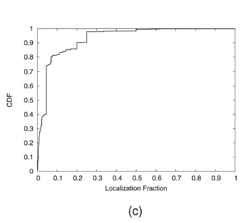
(4) In Fig.4c Subplot shows the localization efficiency defined in Section 5.2.3 over 3,000 real failure events.
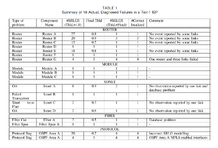
Experience with Real Failure Data
It is able to verify manually that SCORE successfully localized all of the 18 faults studied to the failed network elements (shown in Table 1). However, when a threshold of 1.0 (i.e., mandated that an SRLG can be identified if and only if faults were observed on all corresponding IP links) was used, it was typically unsuccessful— particularly for router failures, and for the protocol bug reported.
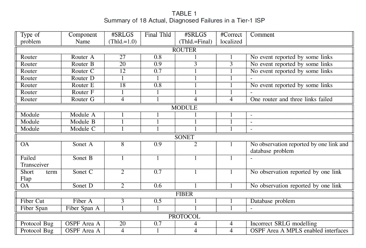
ta
There are four common SONET network element failures . The first—an optical amplifier failure—induced faults on 13 IP links.
The other three SONET failures were all correctly isolated to the SRLG containing the failed network element; in two cases, we again had to lower the threshold used within the algorithm to account for links for which we had no failure notification. In one of these cases, the missing link was indeed a result of the interface having been operationally shut down shortly before the failure.
On another previously identified failure scenario affected by an SRLG database error (fiber A in Table 1), the system was unable to identify a single SRLG as being the culprit even as the threshold was lowered, because no SRLG in the database contained all of the circuits reporting the fault.
The final case that evaluated was one in which a lowlevel protocol implementation problem (software bug) affected a number of links within a common OSPF area.
Localization efficiency

In Fig.4c Subplot shows the localization efficiency defined in Section 5.2.3 over 3,000 real failure events.It is clearly illustrated that the SCORE algorithm can efficiently ferret out likely causes from a large set of possible causes for a given failure.
However,because of the extensive manual labor involved in diagnosing failures, we cannot make sure the true cause of all 3,000 failures and cannot measure accuracy on this data set.
Related work[]
One critical component in applying the risk modeling approach in the LINK FAULT scenario is the construction of SRLGs. Network engineers routinely employ the concept of SRLGs to provision disjoint paths in optical networks, as input into many traffic engineering mechanisms, and in protocols such as Generalized Multiprotocol Label Switching (GMPLS). Due to their importance, previous work has attempted to automatically infer SRLGs in the optical domain. To the best of our knowledge, however, we are first to use SRLGs in combination with higher layer fault notifications to isolate failures in the optical hardware of a network backbone without the need for physical layer monitoring.
Conclusion[]
In this paper, we develop and evaluate a simple but effective method for network fault localization. Our method is based on risk models which can locate the fault, even in the absence of any network generated alarm, either because they are not available, or because of the silence of the nature of the fault, which help network operators fault troubleshooting even when traditional monitoring failed. Although we article discusses two specific situations, there may be many other cases, our method is directly applicable that are remained to be explored. Our extensive evaluation is based on the controlled simulation and an actual failure data,which can acquire high localization accuracy and precision in many failure scenarios.
Reference[]
|
[1] This paper appears in: Dependable and Secure Computing, IEEE Transactions on Date of Publication: Oct.-Dec. 2010 Author(s): Kompella, R.R. Dept. of Comput. Sci., Purdue Univ., West Lafayette, IN, USA Yates, J. ; Greenberg, A. ; Snoeren, A.C. Volume: 7 , Issue: 4 Page(s): 396 - 409 |
[2] P. Sebos, J. Yates, D. Rubenstein, and A. Greenberg, “Effectiveness of Shared Risk Link Group Auto-Discovery in Optical Networks,” Proc. Optical Fiber Comm. Conf., Mar. 2002.